Why Learn Excel

Let me explain Microsoft Excel.

Microsoft Excel is a Microsoft 365 application used for analyses and reporting data. Microsoft Excel has built-in features to perform multitudes of operations like such as Calculations, OLAP cubes, Pivots tables, Charting Dashboard reporting and a complete Rapid Application Development.

Although little recognised, Excel's most powerful feature is connecting to just about any data source currently available, including Websites, APIs, PDFs and anything that contains data. There is no other utility apart from Microsoft Power BI with that versatility

An Excel file called a workbook consists of one or more worksheets (spreadsheets). Further, each worksheet is made up of millions of cells in a massive grid in columns and rows that form a table. Alphabetical letters are usually assigned to columns, and numbers are usually assigned to rows. The point where a column and a row meet is called a cell. The address of a cell is given by the letter representing the column and the number representing a row.

Is it worth your time to  Learn Microsoft Excel?

We all deal with numbers in one way or the other, but we cannot always analyse that data in a succinct matter to make decisions. That is where Excel comes in.

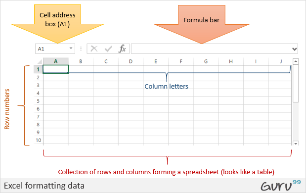
The overall vision of an Excel worksheet can be intimidating to anyone looking at it for the first time. However, if you are familiar with other Microsoft 365 applications it shouldn't be a shock.

 

 

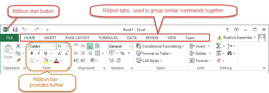
Ribbon components explained

Ribbon start button – is for accessing commands i.e. creating new documents, saving existing work and printing

Ribbon tabs – the tabs are used to group similar commands together. The home tab is used for basic commands such as formatting the data to make it more presentable, and sorting and finding specific data within the spreadsheet.

Ribbon bar – the bars are used to group similar commands together. As an example, the Alignment ribbon bar is used to group all the commands that are used to align data together.

 

Understanding Workbooks, Worksheets, rows and columns.

A worksheet is a collection of rows and columns. When a row and a column meet, they form a cell. Cells are used to record data. Each cell is uniquely identified using a cell address. Columns are usually labelled with letters while rows are usually numbers.

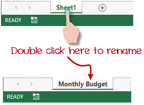
A workbook is a collection of worksheets. By default, a workbook has three cells in Excel. You can delete or add more sheets to suit your requirements. By default, the sheets are named Sheet1, Sheet2 and so on. You can rename the sheet names to more meaningful names i.e. Daily Expenses, Monthly Budget, etc

 

You can customise the Microsoft Excel environment

I like blue as a colour, so you imagine my Excel theme tends to err on bluish. Your favourite colour could be any of the 256 colour schemes. In this sub-section, we are going to look at;

• Customization of the ribbon
• Setting the colour theme
• Settings for formulas
• Proofing settings
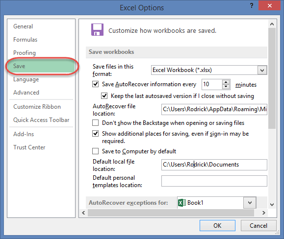
• Save settings

 

The above image shows the default ribbon in Excel 2013. Let’s start with the customisation of the ribbon, suppose you do not wish to see some of the tabs on the ribbon, or you would like to add some tabs that are missing such as the developer tab. You can use the options window to achieve this.

• Click on the ribbon start button
• Select options from the drop-down menu. You should be able to see an Excel Options dialogue window
• Select the customize ribbon option from the left-hand side panel as shown below

 

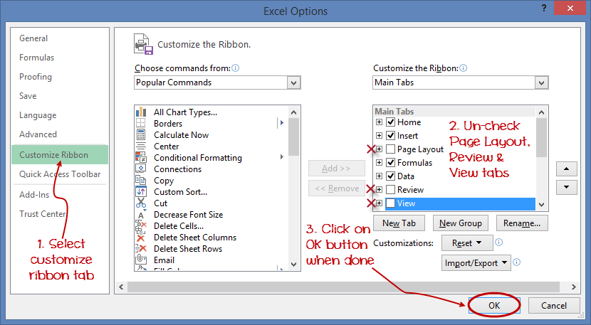
• On your right-hand side, remove the check marks from the tabs that you do not wish to see on the ribbon. For this example, we have removed Page Layout, Review, and View tabs.
• Click on the “OK” button when you are done.

Your ribbon will look as follows:

 

 

Adding your custom tabs to the ribbon

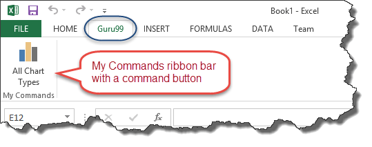
You can also add your tab, give it a custom name and assign commands to it. Let’s add a tab to the ribbon with the text Guru99

 

1. Right-click on the ribbon and select Customize the Ribbon. The dialogue window shown above will appear
2. Click on the new tab button as illustrated in the animated image below
3. Select the newly created tab
4. Click on Rename button
5. Give it the name Guru99
6. Select the New Group (Custom) under the Guru99 tab as shown in the image below
7. Click on Rename button and give it the name of My Commands
8. Let’s now add commands to my ribbon bar
9. The commands are listed on the middle panel
10. Select the All chart types command and click on Add button
11. Click on OK

Your ribbon will look as follows:

Setting the colour theme

To set the colour theme for your Excel sheet you have to go to the Excel ribbon and click on a File Option command. It will open a window where you have to follow the following steps.

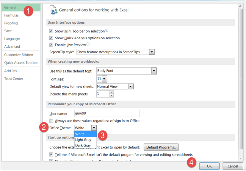
1. The general tab on the left-hand panel will be selected by default.
2. Look for the colour scheme under General options for working with Excel
3. Click on the colour scheme drop-down list and select the desired colour
4. Click on the OK button

Settings for formulas

This option allows you to define how Excel behaves when you are working with formulas. You can use it to set options i.e. autocomplete when entering formulas, change the cell referencing style and use numbers for both columns and rows and other options.

 

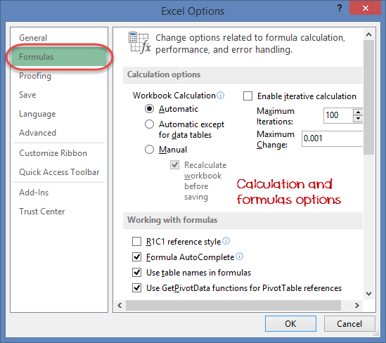
 If you want to activate an option, click on its check box. If you want to deactivate an option, remove the mark from the checkbox. You can this option from the Options dialogue window under the formulas tab from the left-hand side panel.

 

Proofing settings

 

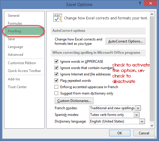
 This option manipulates the entered text entered into Excel. It allows setting options such as the dictionary language that should be used when checking for wrong spellings, suggestions from the dictionary, etc. You can this option from the options dialogue window under the proofing tab from the left-hand side panel.

 

 

 Courtesy of: Guru 99